
Every major open-weight release revives the same prediction: laptops and phones will soon displace the cloud, and AI data centers will cease to matter as much as they do now.
I expect something less tidy. Local AI will grow. Yet the screen where AI appears and the place where its computation happens are separate questions. A small model on a device may begin a conversation, redact sensitive details, or handle a quick command, while long reasoning, large contexts, and tool-heavy jobs move to a data center. More local AI and more data-center inference can grow at the same time.
This is not an argument against local models, nor a claim that the cloud is always cheaper. It is a structural analysis based on official documentation and primary research available on August 25, 2026. It asks where the data center has an advantage and where that advantage disappears. It is not a hands-on speed benchmark or a forecast of market share five years from now.
Open weights are real progress, but “local” is not one deployment class
Open weights mean that the trained parameters can be downloaded and run on infrastructure chosen by the operator. The label does not necessarily mean that the source code and training data are fully open. It also says nothing by itself about the cost of serving the model.
OpenAI’s gpt-oss announcement makes the distinction concrete. The company says gpt-oss-20b was designed to run in 16GB of memory, while gpt-oss-120b fits in 80GB. Both are open-weight models. The first can target a high-end personal device or edge machine; the second requires an 80GB-class GPU or an environment with equivalent memory capacity.
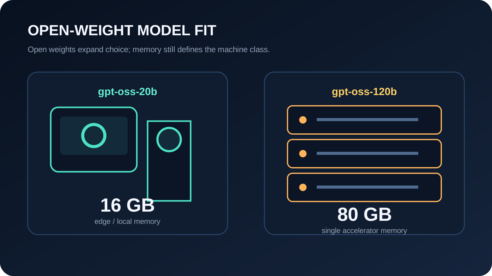
Source figures: OpenAI, Introducing gpt-oss. Checked 2026-08-25. Fitting a model in memory does not establish its speed or quality.
That is why “local versus cloud” is too coarse a starting point. A desktop PC, an on-premises cluster in a company server room, a dedicated GPU rented from a hosting provider, and a model vendor’s API are four different operating choices. An eight-GPU server controlled by one company may be local in an ownership sense, but its power, cooling, and operations already resemble a small data center. Conversely, an open-weight model can be served by a third-party cloud.
Capability is not a fixed finish line either. A small model may catch a larger model on a particular benchmark. That does not show that it will finish tomorrow’s longer agent task at the same cost. Expectations rise as context windows, tool use, error recovery, multimodal input, and the length of a useful run expand. The practical question is not simply how clever the local model has become. It is which model completes the intended job with the fewest retries.
This matters because a model that produces a plausible first answer can still be the expensive option if a person must repeatedly repair its plan, restart its tools, or split a large job into many smaller prompts. Model quality and deployment cost cannot be separated when the unit that matters is a completed task rather than one generated token.
The data center’s strongest advantage is a shared request pool
Owning costly GPUs is only part of the data-center advantage. A large and continuous queue, supplied by many unrelated users, is just as important.
NVIDIA’s Triton documentation describes dynamic batching: a server combines individual inference requests and executes them together. A batch will often improve throughput, but waiting to form a larger batch can increase latency. Operators therefore tune batch size and waiting time against a service’s latency budget.
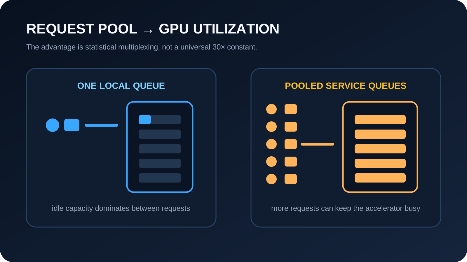
Conceptual basis: NVIDIA Triton Dynamic Batcher. The benefit depends on the model, input lengths, concurrency, and latency target.
Interactive language models generate output tokens sequentially, so they cannot finish every calculation in one pass. Even so, a serving system can interleave token-generation steps from different users on the same accelerator and reduce otherwise empty capacity. A data center is well positioned to do this because requests arrive across customers, applications, time zones, and hours of the day.
Local machines can batch too. A developer running several agents at once, or a company sharing an internal model server across teams, can create useful concurrency. The difference is not whether batching is technically possible. It is how reliably there is another compatible request ready to run. Depreciation continues while one owner sleeps. A large service can fill that interval with demand from elsewhere.
This is statistical multiplexing, not magic. The data center does not make an operation free; it spreads fixed capacity across a broader and less correlated demand pool. The advantage shrinks for a local machine that stays busy doing valuable work. It grows for expensive hardware purchased for occasional bursts.
It is tempting to compress this into a claim such as “the data center is 30 times more efficient.” That would make the case weaker. The PagedAttention paper reported two to four times higher throughput than prior systems at a similar latency level in the workloads the authors tested. That is important evidence for better serving efficiency, but it is not a universal multiplier for every model and GPU. The direction is defensible; the exact ratio must be measured in the target environment.
Cost turns on utilization and equivalent model quality, not just GPU price
A local estimate that includes only electricity is incomplete. An API estimate based only on a monthly subscription is incomplete as well. At minimum, the comparison needs a common accounting boundary:
monthly local TCO = (hardware price - residual value) / months in service
                    + average power × hours used × electricity rate
                    + cooling, failure, and operating costs

monthly API cost = input tokens × input price
                   + output tokens × output price
                   + tool, storage, and network costs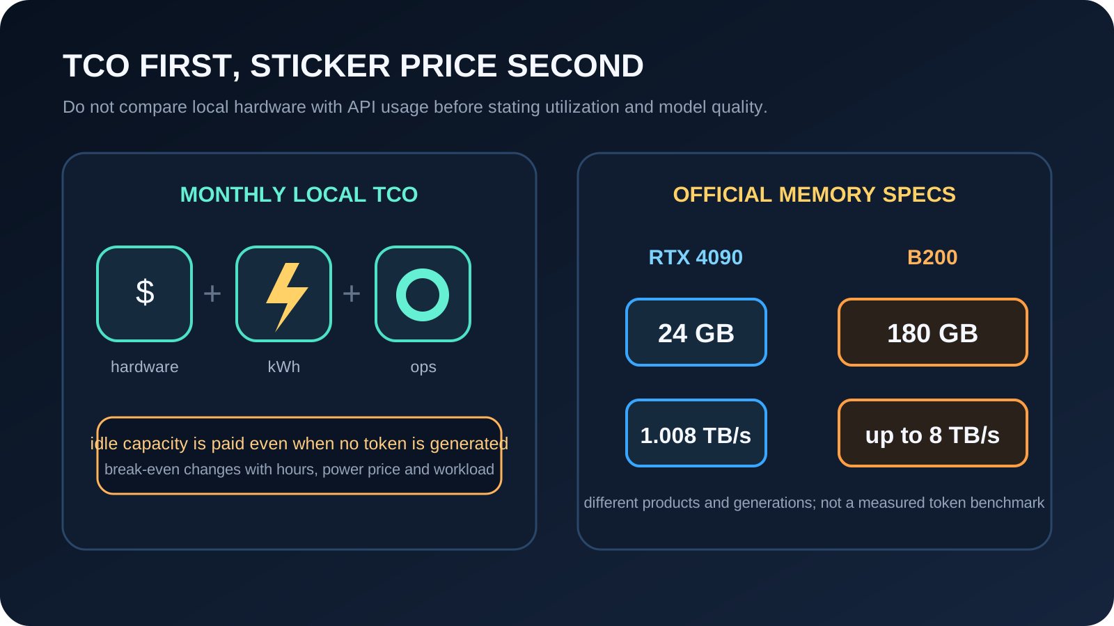
Hardware figures: NVIDIA Ada architecture white paper and NVIDIA HGX AI Factory specifications. These are different generations and product classes, not a direct LLM tokens-per-second benchmark.
NVIDIA’s published specifications list the RTX 4090 with 24GB of GDDR6X memory and 1,008GB/s of memory bandwidth. One B200 has 180GB of HBM3e and up to 8TB/s of bandwidth—about 7.5 times the capacity and 7.9 times the bandwidth. Those figures show that the data-center part was designed to hold larger models and serve more concurrent work. They do not prove that it is exactly 7.9 times faster for every language model. Precision, batch size, context length, and the software stack all affect delivered performance.
The break-even point is personal. If the GPU already exists and useful jobs keep it occupied around the clock, the marginal local cost can be low. If demand arrives in bursts and a stronger model is needed only occasionally, paying for an API may beat purchasing idle capacity. When policy forbids external transfer of the data, cost may not be the first decision at all.
OpenAI’s open-weight guide similarly notes that self-hosting may be cost-effective in some situations, while an API may be more efficient once hosting, maintenance, and related services are included. That conditional answer is more useful than either slogan. Without workload volume and a quality requirement, neither “local is always cheaper” nor “cloud is always cheaper” can be supported.
Model equivalence is the part most cost sheets miss. Comparing a small local model with a stronger cloud model is not fair if the smaller model causes more retries, more review, or a lower completion rate. Comparing them can still be useful, but the unit should be a task completed to the same acceptance threshold. Cheap tokens are not cheap work when they do not finish the job.
There are boundaries where local inference clearly wins
The strongest cases for local inference come from constraints, not taste.
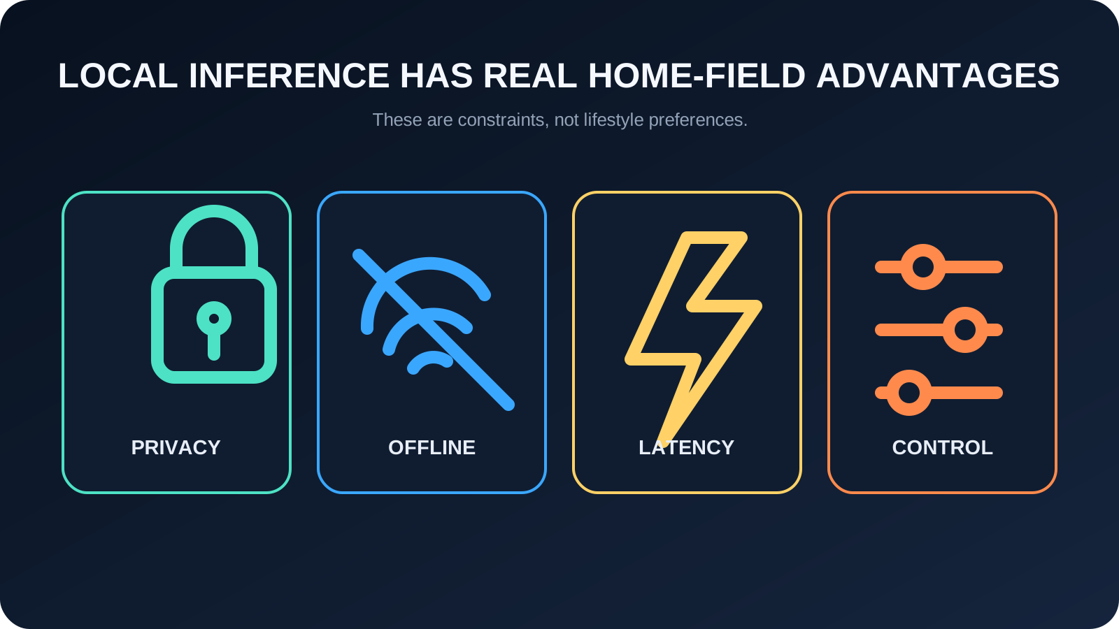
- Data must not leave the environment. In legal, medical, or confidential corporate settings where external APIs are not permitted, owned infrastructure is a requirement rather than a preference.
- The product must work without a reliable connection. On-site equipment, mobile environments, and emergency response need an on-device path that survives a network outage.
- Response time must be short and predictable. Keyboard suggestions, voice interfaces, and camera assistance can suffer when a network round trip sits in the critical path.
- The model and its logs must remain under direct control. Self-hosting open weights helps when an organization must pin a version, customize it, or audit the full data-retention path.
Under those conditions, peak general capability can matter less than reliable execution at the moment of need. A small specialist model that completes one recurring operation consistently may be more valuable than a higher-scoring general model.
Local is not automatically secure, however. Downloaded models and runtimes introduce supply-chain questions. Malware on the PC, local logs and backups, and user permissions remain security concerns. Keeping data away from a cloud service is one layer of privacy protection; it is not a complete security program.
The boundary also changes with workload shape. A video workstation that performs useful inference every night is not comparable to a laptop that wakes a model twice a week. A factory with an internal request pool may capture much of the utilization advantage normally associated with the cloud. “Local” should describe the operating conditions, not serve as a proxy for small or inefficient.
The likely future is hybrid routing, not one winner
Products are already combining local and cloud execution. Apple’s Private Cloud Compute documentation describes a system in which suitable requests run on the device while those requiring a more capable foundation model go to cloud infrastructure. Android’s experimental hybrid inference API can prefer on-device Gemini Nano and fall back to the cloud when it is unavailable, or prefer the cloud and fall back to the device when offline.
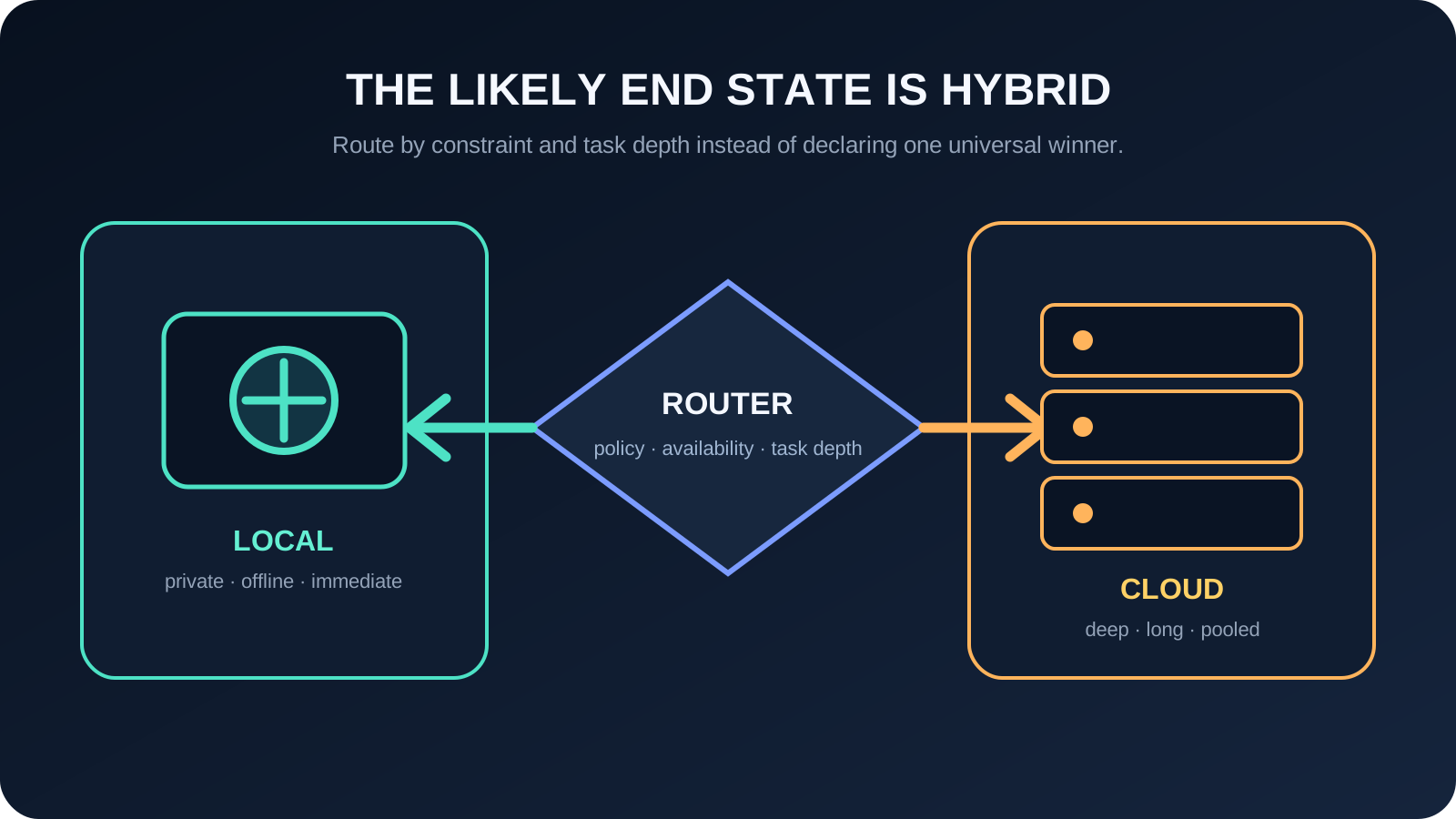
Implementation examples: Apple Private Cloud Compute and Android experimental hybrid inference. The Android feature was experimental as of 2026-08-25.
The Interaction Models essay from Thinking Machines offers another useful separation of roles. A real-time interaction model stays responsive to the user, while deeper reasoning and tool use can be assigned to an asynchronous background model. This is evidence for separating a fast model from a deep model, not proof that the first is local and the second is in the cloud. Conflating the two would overstate the source.
My working expectation is that a device model will clean inputs, redact private information, provide short immediate responses, and retain basic functionality offline. Server models will handle long documents, large codebases, complex tool calls, and decisions with a high quality threshold. The customer will experience one product, while several models and execution locations divide the work behind it.
Five routing questions cover most of the decision:
| Question | Leans local | Leans data center |
|---|---|---|
| May the data leave the device or premises? | Transfer prohibited or sensitive | Transfer permitted by policy |
| Is the internet always available? | Offline operation required | Stable connection available |
| How long can the user wait? | Immediate response required | Longer processing acceptable |
| How deep and long is the task? | Short and repetitive | Long context and complex tools |
| How consistently can requests fill capacity? | High fixed utilization | Variable demand or large concurrency |
Several developments could prove this outlook wrong. Small-model quality might rise much faster than user expectations. Memory and energy efficiency might improve dramatically. Regulation might make external data centers impractical. In the other direction, AI jobs could keep becoming longer and more complex, strengthening centralization. None of those paths is settled today.
The present structure still supports a clear conclusion: open weights expand the choice of execution location, but they do not remove the economics of pooling requests and sharing large memory and accelerators. My structural expectation is that local AI will grow while a substantial share of aggregate compute remains in data centers, with the user’s device becoming the first layer that decides when to call it.
Write these down before choosing a deployment location
- Confirm that the models being compared deliver equivalent task quality.
- Measure monthly input and output tokens, as well as concurrent request volume.
- Include depreciation, electricity, cooling, and operating time in local cost.
- Resolve privacy and data-residency requirements before optimizing the cost sheet.
- Define a fallback for both local failure and cloud failure.
- Revisit routing by task instead of treating one location as permanent.
This analysis relies on official documentation and primary research. It cannot substitute for a benchmark of a specific model or for an organization’s own cost base. Before committing, run a short local-versus-API measurement with the same prompts, the same quality threshold, and the same workload.
References and reporting
Public pages used for reported facts, official documentation, policy background, product details, and claims that may change.
- Introducing gpt-ossOpenAIUsed for: memory requirements for gpt-oss-20b and gpt-oss-120b; distinguishing open weights from the hosting environmentChecked: 2026-08-25
- OpenAI open-weight modelsOpenAIUsed for: when self-hosting costs can make sense; data control and customization benefitsChecked: 2026-08-25
- Triton dynamic batcherNVIDIAUsed for: definition of dynamic batching; the throughput-latency trade-offChecked: 2026-08-25
- Efficient Memory Management for Large Language Model Serving with PagedAttentionUC BerkeleyUsed for: memory management in LLM serving; throughput gains within the paper's experimental scopeChecked: 2026-08-25
- NVIDIA Ada GPU ArchitectureNVIDIAUsed for: RTX 4090 memory capacity; memory bandwidth and maximum board powerChecked: 2026-08-25
- NVIDIA HGX AI Factory componentsNVIDIAUsed for: B200 memory capacity; B200 memory bandwidthChecked: 2026-08-25
- Private Cloud Compute Security GuideAppleUsed for: division of work between on-device and cloud execution; privacy design for cloud processingChecked: 2026-08-25
- Experimental hybrid inference and new Gemini models for AndroidGoogle Android DevelopersUsed for: hybrid local-cloud inference; on-device preference with cloud fallbackChecked: 2026-08-25
- Interaction ModelsThinking Machines LabUsed for: separating a real-time interaction model from a background model; limits of treating model-role separation as local-cloud evidenceChecked: 2026-08-25